Advanced NumPy
%matplotlib inline
Quick example: gene expression, without numpy
FIRST...
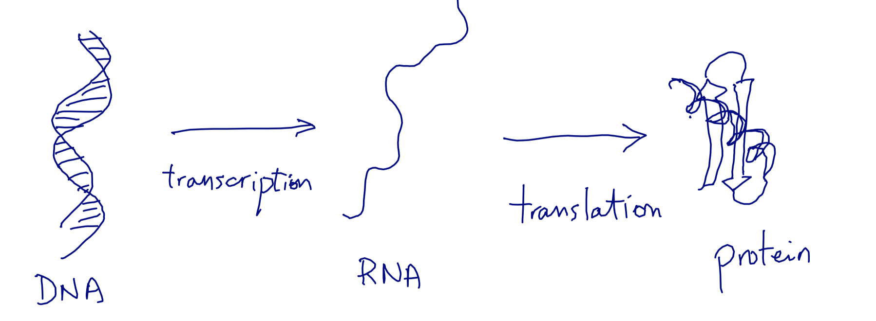
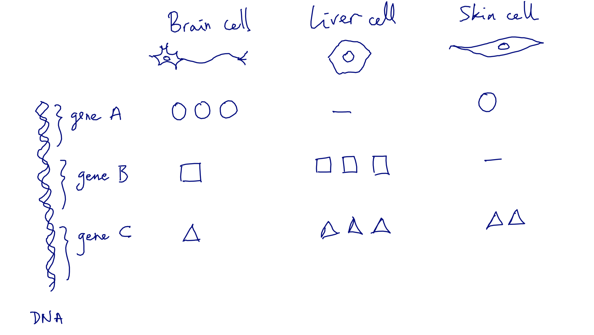
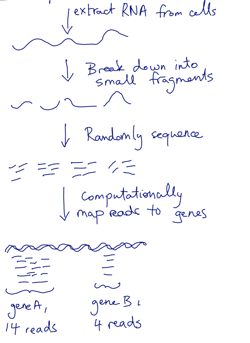
Some fake data
| | Cell type A | Cell type B | Cell type C | Cell type D | |——–|————-|————-|————-|————-| | Gene 0 | 100 | 200 | 50 | 400 | | Gene 1 | 50 | 0 | 0 | 100 | | Gene 2 | 350 | 100 | 50 | 200 |
gene0 = [100, 200, 50, 400]
gene1 = [50, 0, 0, 100]
gene2 = [350, 100, 50, 200]
expression_data = [gene0, gene1, gene2]
Why is this a bad idea?
Now with NumPy
import numpy as np
a = np.array(expression_data)
print(a)
[[100 200  50 400]
 [ 50   0   0 100]
 [350 100  50 200]]
We are going to:
- Obtain an RPKM expression matrix
- Quantile normalize the data
using the awesome power of NumPy
Inside a numpy ndarray
def print_info(a):
    print('number of elements:', a.size)
    print('number of dimensions:', a.ndim)
    print('shape:', a.shape)
    print('data type:', a.dtype)
    print('strides:', a.strides)
    print('flags:', a.flags)

print_info(a)
number of elements: 12
number of dimensions: 2
shape: (3, 4)
data type: int64
strides: (32, 8)
flags:   C_CONTIGUOUS : True
  F_CONTIGUOUS : False
  OWNDATA : True
  WRITEABLE : True
  ALIGNED : True
  UPDATEIFCOPY : False
print(a.data)
<memory at 0x7fa0e836d7e0>
abytes = a.ravel().view(dtype=np.uint8)
print_info(abytes)
number of elements: 96
number of dimensions: 1
shape: (96,)
data type: uint8
strides: (1,)
flags:   C_CONTIGUOUS : True
  F_CONTIGUOUS : True
  OWNDATA : False
  WRITEABLE : True
  ALIGNED : True
  UPDATEIFCOPY : False
print(abytes[:24])
[100   0   0   0   0   0   0   0 200   0   0   0   0   0   0   0  50   0
   0   0   0   0   0   0]
Example: take the transpose of a
print_info(a)
number of elements: 12
number of dimensions: 2
shape: (3, 4)
data type: int64
strides: (32, 8)
flags:   C_CONTIGUOUS : True
  F_CONTIGUOUS : False
  OWNDATA : True
  WRITEABLE : True
  ALIGNED : True
  UPDATEIFCOPY : False
print_info(a.T)
number of elements: 12
number of dimensions: 2
shape: (4, 3)
data type: int64
strides: (8, 32)
flags:   C_CONTIGUOUS : False
  F_CONTIGUOUS : True
  OWNDATA : False
  WRITEABLE : True
  ALIGNED : True
  UPDATEIFCOPY : False
Example: skipping rows and columns with slicing
print_info(a.T)
number of elements: 12
number of dimensions: 2
shape: (4, 3)
data type: int64
strides: (8, 32)
flags:   C_CONTIGUOUS : False
  F_CONTIGUOUS : True
  OWNDATA : False
  WRITEABLE : True
  ALIGNED : True
  UPDATEIFCOPY : False
print_info(a.T[::2])
number of elements: 6
number of dimensions: 2
shape: (2, 3)
data type: int64
strides: (16, 32)
flags:   C_CONTIGUOUS : False
  F_CONTIGUOUS : False
  OWNDATA : False
  WRITEABLE : True
  ALIGNED : True
  UPDATEIFCOPY : False
print_info(a.T[::2, ::2])
number of elements: 4
number of dimensions: 2
shape: (2, 2)
data type: int64
strides: (16, 64)
flags:   C_CONTIGUOUS : False
  F_CONTIGUOUS : False
  OWNDATA : False
  WRITEABLE : True
  ALIGNED : True
  UPDATEIFCOPY : False
Getting a copy
b = a
print(b)
[[100 200  50 400]
 [ 50   0   0 100]
 [350 100  50 200]]
a[0, 0] = 5
print(b)
a[0, 0] = 100
[[  5 200  50 400]
 [ 50   0   0 100]
 [350 100  50 200]]
Advanced operations: axis-wise evaluation
expr = np.load('../../data/expr.npy')
print_info(expr)
number of elements: 7687500
number of dimensions: 2
shape: (20500, 375)
data type: uint32
strides: (4, 82000)
flags:   C_CONTIGUOUS : False
  F_CONTIGUOUS : True
  OWNDATA : False
  WRITEABLE : True
  ALIGNED : True
  UPDATEIFCOPY : False
This has the raw read count data. However, each sample gets a different number of reads, so we want to normalize by the library size, which is the total number of reads across a column.
The np.sum function returns the sum of all the elements of an array. With the axis argument, you can take the sum along the given axis.
lib_size = np.sum(expr, axis=0)
print(lib_size)
[ 41539237  50824374  35747651  33532890  48162893  83478927  61652756
  56043182  50066035  44291909  62103960  52177691  39935196  44712296
  49499950  54994779  64874312  41901128  61124396  74947233  55805778
  44751480  57419892  45460279  58590618  75900141  79022684  51253368
  63148322  64114541  53696942  50946576  55709927  60184139  73887491
  51905092  39721522  42746126  43019952  40435776  57789966  30526018
  50488171  59600438  49802751 103219262  80445758  76730579  59996715
  70611975  53788477  57967905  50450027  61725636  52939093  48355220
  60814140  61419740  52865931  42718020  47981997  50989994  55265609
  57268101  37174525  65469319  69459796  64633280  52550614  52800398
  67603908  42568697  54328614  58801154  41408022  55721943  56051351
  48906539  30074621  56514800  61685565  45155573  55190918  58239673
  51484868  56456500  58897501  41200475  60510647  45186472  48863100
  44723293  66857959  43679229  63454731  40459554  44210528  71649897
  51052494  55893243  23880954  37930574  50358271  67084571  55954779
  60533989  37534918  58268372  69034028  62187943  31471960  60211327
  69060349  52800469  54351395  48929065  55783836  57805383  45280443
  64365686  51738764  45503686  20805588   6231205  58912016  58382737
  55586370  47844506  88199645  45202180  57012734  35536183  66413476
  58255198  67400957  63388779  66920588  89665770  54467447  53674778
  60489113  64271298  54482571  57945567  58481866  30468523  46520205
  43720270  20860933  62291312  76469475  58273889  62758553  69907767
  46323880  58981816  57005722  63065832  55354924  53218346  48332445
  50847760  45896941  50855098  66765635  53976120  43076562  64591516
  70321285  43164571  19972560  60273622  48626910  62192138  56940941
  54212832  47915415  60829977  64420702  47877190  21861554  42351337
  56078062  58080584  65786195  69711708  35936611  61273004  40872795
  42664688  51610919  42895450  65840053  46914753  52775804  48278133
  63447113  46209355  46190947  55448740  40136288  61288618  55819950
  61874813  51645078  52880150  56670662  41643222  54351160  38218219
  20136141  48512044  54430430  40095409  37135634  47338323  47628500
  70593750  61983198  33989258  62762404  32312231  54883550  58804271
  47618042  43385504  53262000  51775467  77796207  60667212  58663579
  48561056  37776295  41013665  61718896  49617862  46246248  53495544
  59868475  65570441  57271936  33651719  42949256  56326986  46188444
  65338751  63280380  72026286  45558125  65005023  37707710  36690847
  36791707  47339679  40636949  47695871  59847402  65956305  59465169
  70009556  58111425  60158442  54800853  54455853  68528086  44581634
  45475847  66490471  42291085  35965990  41479598  58860157  36363286
  43083690  59348176  58854511  41230056  49617871  43539028  65823859
  44602672  50578213  57054596  45886960  66240091  66165612  32463206
  47864659  52971575  52220505  25097393  70434480  32039712  32819373
  58584329  45039848  59657923  49474656  63730127  65560607  47372745
  58633031  63905299  54165552  47486106  52398513  45153699  58159323
  19581961  66938365  70099565  62639887  34726837  63115934  69049347
  66656207  44194958  43770898  63897405  32572188  21661735  40549383
  37659411  45886025  64801505  21061525  59949050  31486861  62661761
  49585558  61242121  69353546  60024113  58447218  61229433  44275809
  64901114  37277569  36078563  44834451  62844105  53060365  66203234
  63269672  52694324  61885104  51421981  59063240  43349098  48320365
  89431418  40367656  61502892  64771848  36282255  45373426  66499413
  56130605  40281506  45002236  55357976  61842699  30509789  43349038
  59621075  69058739  67386247  55079081  28732898  56053773  60685111
  39380186  45394727  59700010  54182166]
Exercise
Generate a 10 x 3 array of random numbers. From each row, pick the number closest to 0.75. Make use of np.abs and np.argmax to find the column j which contains the closest element in each row.
Advanced operations: broadcasting
In order to normalize every column by its corresponding library size, we have to align the two arrays’ axes: each dimension must be either the same size, or one of the arrays must have size 1. Use np.newaxis to match the dimensions.
print(expr.shape)
print(lib_size.shape)
print(lib_size[np.newaxis, :].shape)
(20500, 375)
(375,)
(1, 375)
However, NumPy will automatically prepend singleton dimensions until the array shapes match or there is an error:
np.all(expr / lib_size ==
       expr / lib_size[np.newaxis, :])
True
expr_lib = expr / lib_size
We also multiply by $10^6$ in order to keep the numbers on a readable scale (reads per million reads).
expr_lib *= 1e6
Finally, longer genes are more likely to produce reads. So we normalize by the gene length (in kb) to produce a measure of expression called Reads Per Kilobase per Million reads (RPKM).
gene_len = np.load('../../data/gene-lens.npy')
print(gene_len.shape)
(20500,)
Exercise: broadcast expr_lib and gene_len together to produce RPKM
rpkm = expr_lib # FIX THIS
import matplotlib.pyplot as plt
from scipy import stats

def plot_col_density(data, xlim=None, *args, **kwargs):
    # Use gaussian smoothing to estimate the density
    density_per_col = [stats.kde.gaussian_kde(col) for col in data.T]
    if xlim is not None:
        m, M = xlim
    else:
        m, M = np.min(data), np.max(data)
    x = np.linspace(m, M, 100)

    fig, ax = plt.subplots()
    for density in density_per_col:
        ax.plot(x, density(x), *args, **kwargs)
    ax.set_xlabel('log-counts')
    ax.set_ylabel('frequency')
    if xlim is not None:
        ax.set_xlim(xlim)
    plt.show()
%matplotlib inline
plt.style.use('ggplot')
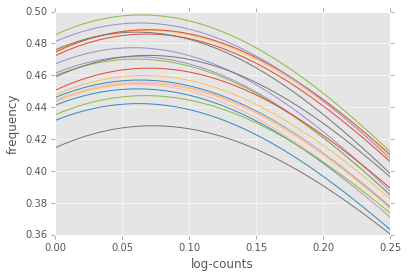
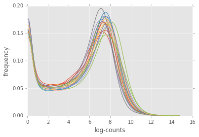
plot_col_density(np.log(expr+1)[:, :20])
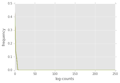
plot_col_density(np.log(rpkm + 1)[:, :20], xlim=(0, 250))
Exercise: 3D broadcasting
Below, produce the array containing the sum of every element in x with every element in y
x = np.random.rand(3, 5)
y = np.random.randint(10, size=8)
z = x # FIX THIS
Fancy indexing
You can index arrays with slicing, but also with boolean arrays (including broadcasting!), integer arrays, and individual indices along multiple dimensions.
values = np.array([0, 5, 99])
selector = np.random.randint(0, 3, size=(3, 4))
print(selector)
print(values[selector])
[[0 2 1 2]
 [2 0 1 2]
 [2 0 1 0]]
[[ 0 99  5 99]
 [99  0  5 99]
 [99  0  5  0]]
Exercise: quantile normalization
Quantile Normalization(https://en.wikipedia.org/wiki/Quantile_normalization) is a method to align distributions. Implement it using NumPy axis-wise operations and fancy indexing.
Hint: look for documentation for scipy.mstats.rankdata, np.sort, and np.argsort.
def qnorm(x):
    """Quantile normalize an input matrix.

    Parameters
    ----------
    x : 2D array of float, shape (M, N)
        The input data, with each column being a
        distribution to normalize.

    Returns
    -------
    xn : 2D array of float, shape (M, N)
        The normalized data.
    """
    xn = np.copy(x) # replace this by normalizing code
    return xn
logexpr = np.log(expr + 1)
logrpkm = np.log(rpkm + 1)
logexprn = qnorm(logexpr)
logrpkmn = qnorm(logrpkm)
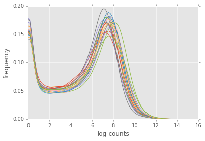
plot_col_density(logexprn[:, :20])
plot_col_density(logrpkmn[:, :20], xlim=(0, 0.25))